This page will consist of instructions on how to make LaTeX accessible (a typesetting language used for research papers; particularly in STEM), along with best practices. The training will be split into the following sections:
- Overview
- LaTeX Best Practices and Authoring Rules
- LaTeX Accessibility Workflow
- Examples by Discipline
- Additional Resources
This training assumes you are already using LaTeX/TeX to author your materials, and serves as a guide for integrating accessibility standards into your current workflow.
If you are new to LaTeX and looking to learn more or get started, visit The LaTeX Project for an overview and basic examples.
Overview
The key components of this workflow are LaTeX and NVDA:
- LaTeX – a typesetting language used for technical and scientific documentation; these are .tex files that typically get converted into PDFs
- NVDA (NonVisual Desktop Access) – a free, open-source, portable screen reader for the Microsoft Windows operating system. This enables blind and vision-impaired individuals to use computers by translating the information on the screen into synthetic speech or braille.
What is the goal of this training?
The goal is to write LaTeX that can become semantic HTML with MathML in order to be accessible for NVDA screenreaders. This training will help with:
- Showing researchers how to prepare LaTeX/TeX source for accessible conversion.
- Converting STEM content into HTML5 with MathML (using Pandoc) so NVDA can read and navigate math continuously.
- Demonstrating accessible text, equations, tables, charts, diagrams, and long descriptions.
- Providing a workflow that can be posted on the website and used by faculty in classrooms.
Why does this workflow matter?
- A visual equation is not enough for screen reader access.
- The source file must preserve structure: headings, lists, tables, captions, links, and math.
- HTML5 with MathML gives assistive technology semantic math to read and navigate.
- The final test is not only visual appearance; it is whether NVDA reads the content correctly.
Overview of Recommended Workflow
- Researcher writes accessible LaTeX
- Keep images, data, captions, and descriptions with the source files
- Convert to HTML5 + MathML using Pandoc
- Test with NVDA in Firefox or Chrome
- Publish HTML and provide source files for review
- Convert the HTML5 to PDF (optional)
LaTeX Best Practices and Authoring Rules
As mentioned, the goal is to author accessible LaTeX source code that converts seamlessly into semantic HTML with MathML, ensuring full accessibility for NVDA screen reader users. Note the following best practices and top 10 authoring rules when working with LaTeX to ensure accessibility. This section corresponds to step 1 of the Recommended Workflow (writing accessible LaTeX)
Top Best Practices for Researchers
- Use sectioning commands such as
\sectionand\subsectionfor structure. - Use real LaTeX math commands; do not insert equation screenshots.
- Use captions for every figure and table.
- Write long descriptions for charts, maps, diagrams, and complex images.
- Use true data tables, not tables for visual layout.
- Use descriptive links instead of “click here.”
- Avoid custom macros unless the conversion workflow has been tested.
Below is an example of an accessible LaTeX snippet.
\section{Calculus Examples}

A derivative can be defined using a limit:
\begin{equation}
f'(x) = \lim_{h \to 0} \frac{f(x+h)-f(x)}{h}.
\end{equation}
Use standard LaTeX syntax whenever possible so the converter can produce clean MathML.
Authoring Rules
Rule 1: Start With a Clean Standard Preamble
The converter understands predictable LaTeX better than heavily customized LaTeX. The preamble should support structure and links, not hide meaning inside style commands. Use common packages and avoid unusual setup when the goal is accessible conversion.
- Use standard document classes and common packages whenever possible.
- Keep layout packages simple; visual formatting should not carry meaning.
- Use hyperref for real links, but make the visible link text descriptive.
- Avoid custom macros until the conversion workflow has been tested.
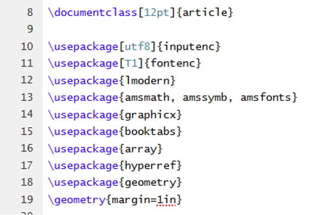
Copyable Code Snippet:
\documentclass[12pt]{article}

\usepackage[utf8]{inputenc}
\usepackage[T1]{fontenc}
\usepackage{lmodern}
\usepackage{amsmath, amssymb, amsfonts}
\usepackage{graphicx}
\usepackage{booktabs}
\usepackage{array}
\usepackage{hyperref}
\usepackage{geometry}
\geometry{margin=1in}
Rule 2: Write Math as Real LaTeX
The rule is simple: if it is math, write it as math. That is what allows Pandoc or LaTeXML to create MathML that NVDA can read and navigate. Equations should be source math, not screenshots or pasted images.
- Use equation environments for displayed equations.
- Use semantic math commands such as \lim, \frac, \sqrt, \int, and \sum.
- Do not replace equations with images just because they look correct visually.
- Keep explanatory sentences before or after equations so the reader has context.
- NVDA should read inline math inside the sentence flow.
- Displayed equations should be announced as math, not images.
- Cases and inequalities should be read in a logical order.
- Use ClearSpeak + Medium verbosity for a clearer demo voice when testing Math content.
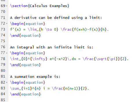
Copyable Code Snippet:
\section{Calculus Examples}

A derivative can be defined using a limit:
\begin{equation}
f'(x) = \lim_{h \to 0} \frac{f(x+h)-f(x)}{h}.
\end{equation}

An integral with an infinite limit is:
\begin{equation}
\int_{0}^{\infty} e^{-x^2}\,dx = \frac{\sqrt{\pi}}{2}.
\end{equation}

A summation example is:
\begin{equation}
\sum_{i=1}^{n} i = \frac{n(n+1)}{2}.
\end{equation}
Rule 3: Use Section Headings for Structure
A screen reader user can jump by heading. That only works if the LaTeX source uses real sectioning commands instead of visual formatting. Headings become navigation points in the final HTML output.
- Use \section and \subsection for document organization.
- Do not create headings by manually bolding or enlarging plain text.
- Write section titles that describe the topic, such as “Vectors and Matrices.”
- Place the explanation before complex notation so users know what they are about to hear.
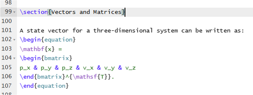
Copyable Code Snippet:
\section{Vectors and Matrices}

A state vector for a three-dimensional system can be written as:
\begin{equation}
\mathbf{x} =
\begin{bmatrix}
p_x & p_y & p_z & v_x & v_y & v_z
\end{bmatrix}^{\mathsf{T}}.
\end{equation}
Rule 4: Use Standard Matrix Environments
Matrix structure should be expressed with rows, columns, and standard delimiters. The converter can only preserve matrix structure when the source marks up the matrix structure. Visually aligned text is not enough.
- Use environments such as bmatrix for matrix notation.
- Use ampersands for columns and double backslashes for rows.
- Do not draw matrices using spaces or images.
- Define the variables around the equation so the notation has meaning.
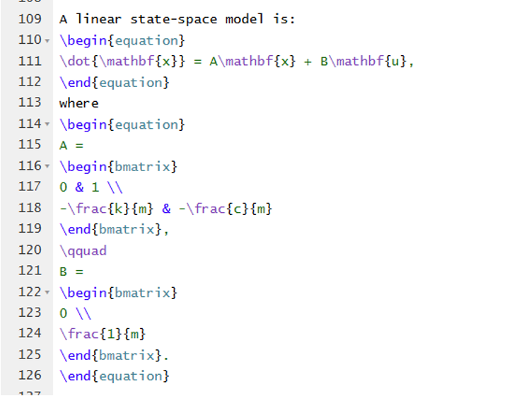
Copyable Code Snippet:
A linear state-space model is:
\begin{equation}
\dot{\mathbf{x}} = A\mathbf{x} + B\mathbf{u},
\end{equation}
where
\begin{equation}
A =
\begin{bmatrix}
0 & 1 \\
-\frac{k}{m} & -\frac{c}{m}
\end{bmatrix},
\qquad
B =
\begin{bmatrix}
0 \\
\frac{1}{m}
\end{bmatrix}.
\end{equation}
Rule 5: Use Cases for Piecewise Functions
When the cases environment is used, NVDA can move through the piecewise function in a logical order. A screenshot of the same function would lose that structure. Piecewise logic needs a real cases environment, not a visual table or screenshot.
- Use the cases environment for piecewise definitions.
- Write each condition explicitly, such as u > u_max.
- Keep inequalities as LaTeX symbols instead of plain visual approximations.
- Explain what the function represents before showing the equation.
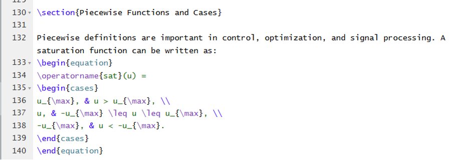
Copyable Code Snippet:
\section{Piecewise Functions and Cases}

Piecewise definitions are important in control, optimization, and signal processing. A saturation function can be written as:
\begin{equation}
\operatorname{sat}(u) =
\begin{cases}
u_{\max}, & u > u_{\max}, \\
u, & -u_{\max} \leq u \leq u_{\max}, \\
-u_{\max}, & u < -u_{\max}.
\end{cases}
\end{equation}
Rule 6: Define Symbols Near the Equation
Greek letters and control notation must be explained in surrounding text. Accessibility is not only about whether NVDA can pronounce symbols. The paper should also explain what those symbols mean when they first appear.
- Use standard commands for Greek letters and notation.
- After an equation, define symbols such as P, Γ, and θ tilde.
- Do not rely on the reader already knowing every symbol.
- Use plain language to connect the equation to the research meaning.
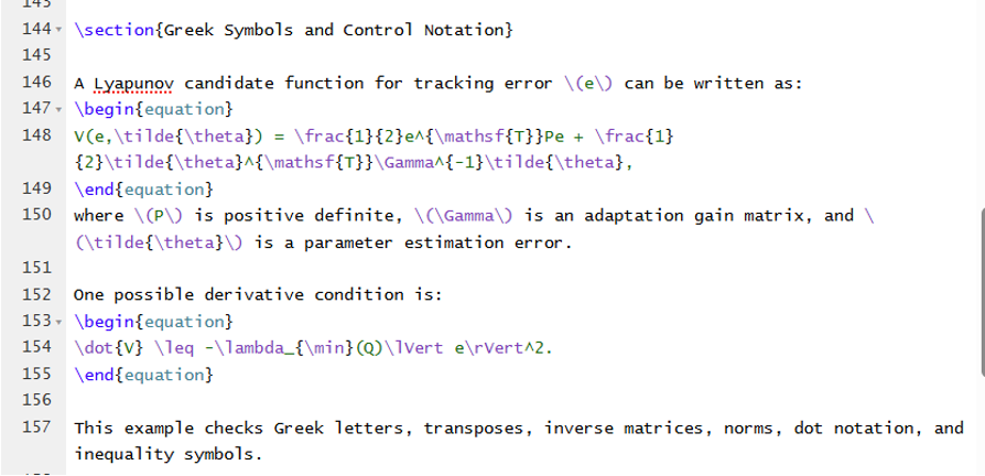
Copyable Code Snippet:
\section{Greek Symbols and Control Notation}

A Lyapunov candidate function for tracking error \(e\) can be written as:
\begin{equation}
V(e,\tilde{\theta}) = \frac{1}{2}e^{\mathsf{T}}Pe + \frac{1}{2}\tilde{\theta}^{\mathsf{T}}\Gamma^{-1}\tilde{\theta},
\end{equation}
where \(P\) is positive definite, \(\Gamma\) is an adaptation gain matrix, and \(\tilde{\theta}\) is a parameter estimation error.

One possible derivative condition is:
\begin{equation}
\dot{V} \leq -\lambda_{\min}(Q)\lVert e\rVert^2.
\end{equation}
Rule 7: Keep Math Inside Lists Semantic
Lists should remain lists even when each item contains equations. If the LaTeX source uses a real list, the HTML output can preserve that list. That helps users understand process steps, algorithms, and procedures.
- Use enumerate or itemize for real list structure.
- Keep each step as a separate item so screen readers announce list position.
- Use inline math inside list items when the equation belongs to the sentence.
- Avoid using manual numbering typed into paragraphs.
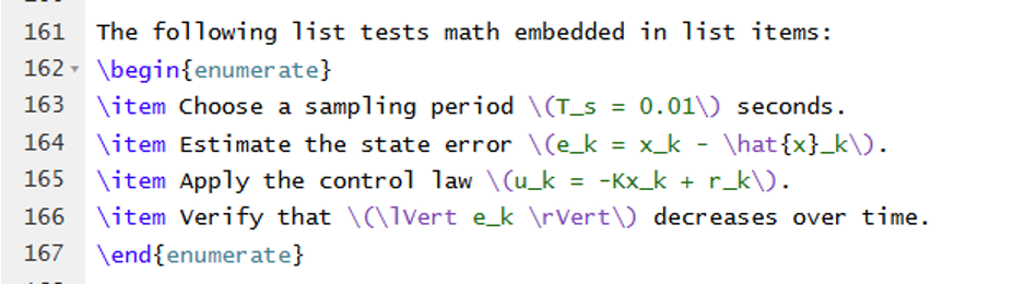
Copyable Code Snippet:
The following list tests math embedded in list items:
\begin{enumerate}
\item Choose a sampling period \(T_s = 0.01\) seconds.
\item Estimate the state error \(e_k = x_k - \hat{x}_k\).
\item Apply the control law \(u_k = -Kx_k + r_k\).
\item Verify that \(\lVert e_k \rVert\) decreases over time.
\end{enumerate}
Rule 8: Create True Data Tables
A table is accessible when a reader can connect each cell to its header. The source should make the table simple and predictable before conversion. Tables need headers and should be used for data, not page layout.
- Use a tabular environment for data with consistent rows and columns.
- Include a caption that explains the table purpose.
- Use a clear header row: Parameter, Symbol, Value, Meaning.
- Avoid merged, nested, or layout-only tables when possible.
- Do not rely on visual spacing to communicate relationships.
- Test table navigation with T and Ctrl + Alt + arrow keys in NVDA.
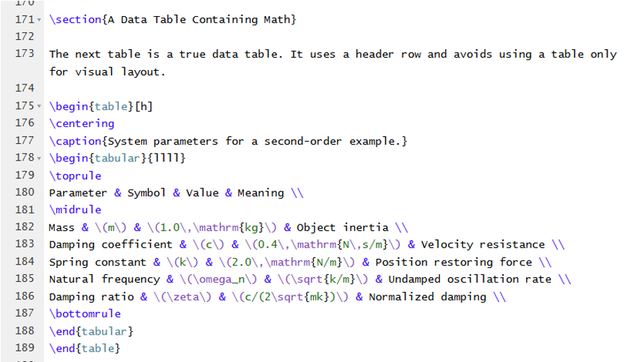
Copyable Code Snippet:
\section{A Data Table Containing Math}

The next table is a true data table. It uses a header row and avoids using a table only for visual layout.

\begin{table}[h]
\centering
\caption{System parameters for a second-order example.}
\begin{tabular}{llll}
\toprule
Parameter & Symbol & Value & Meaning \\
\midrule
Mass & \(m\) & \(1.0\,\mathrm{kg}\) & Object inertia \\
Damping coefficient & \(c\) & \(0.4\,\mathrm{N\,s/m}\) & Velocity resistance \\
Spring constant & \(k\) & \(2.0\,\mathrm{N/m}\) & Position restoring force \\
Natural frequency & \(\omega_n\) & \(\sqrt{k/m}\) & Undamped oscillation rate \\
Damping ratio & \(\zeta\) & \(c/(2\sqrt{mk})\) & Normalized damping \\
\bottomrule
\end{tabular}
\end{table}
Rule 9: Give Charts a Text Equivalent
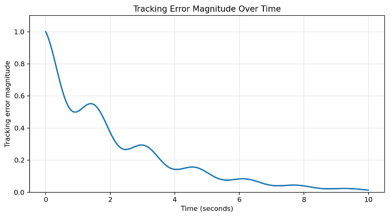
A chart should have a caption, a long description, and data when the data matters. For charts, the goal is not to describe every pixel. The goal is to provide the same academic meaning: what the chart shows, what changes, and what conclusion the reader should take away.
- Use a figure caption for the visible chart.
- Provide a long description that states the trend and main takeaway.
- Add a data table when exact values are important.
- Do not expect alt text alone to explain a complex chart.
- Text equivalents for charts and diagrams – when to use what:
- Use alt text for the short identification of the image.
- Use a figure caption for visible and structural context.
- Use a long description when the image contains important data or relationships.
- For charts, also provide the key data or a linked data table when needed.
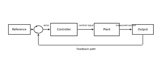
The examples below include a chart and a diagram, which should include a figure caption and a long description as the text equivalents, respectively.
Copyable Code Snippet:
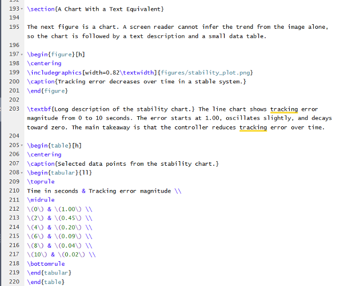
\section{A Chart With a Text Equivalent}

The next figure is a chart. A screen reader cannot infer the trend from the image alone, so the chart is followed by a text description and a small data table.

\begin{figure}[h]
\centering
\includegraphics[width=0.82\textwidth]{figures/stability_plot.png}
\caption{Tracking error decreases over time in a stable system.}
\end{figure}

\textbf{Long description of the stability chart.} The line chart shows tracking error magnitude from 0 to 10 seconds. The error starts at 1.00, oscillates slightly, and decays toward zero. The main takeaway is that the controller reduces tracking error over time.
Rule 10: Explain Block Diagrams in Text
A block diagram needs a written path through the system. When teaching diagrams, explain the process in order. A reader needs the same functional relationship that a sighted reader gets from the arrows.
- Use the figure for sighted users and a text equivalent for screen reader users.
- Describe the flow: input, summing junction, controller, plant, output, feedback.
- Keep the long description close to the figure in the source file.
- Avoid relying only on arrows or spatial position to communicate meaning.
Copyable Code Snippet:
\section{A Block Diagram With a Text Equivalent}

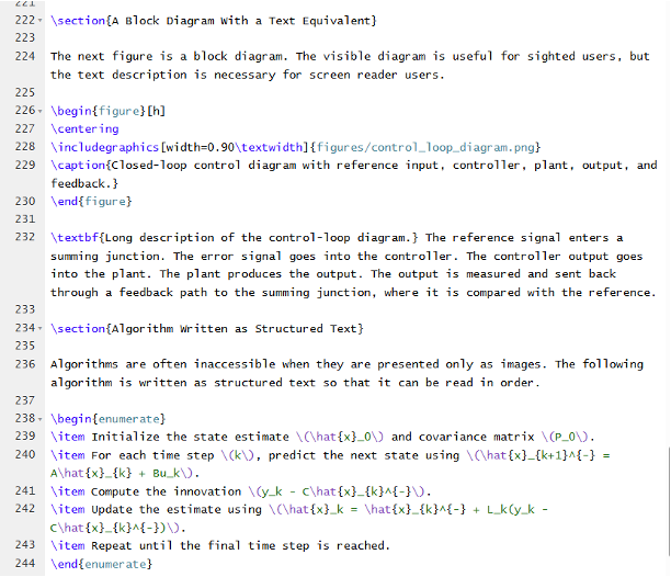
The next figure is a block diagram. The visible diagram is useful for sighted users, but the text description is necessary for screen reader users.

\begin{figure}[h]
\centering
\includegraphics[width=0.90\textwidth]{figures/control_loop_diagram.png}
\caption{Closed-loop control diagram with reference input, controller, plant, output, and feedback.}
\end{figure}

\textbf{Long description of the control-loop diagram.} The reference signal enters a summing junction. The error signal goes into the controller. The controller output goes into the plant. The plant produces the output. The output is measured and sent back through a feedback path to the summing junction, where it is compared with the reference.
LaTeX Accessibility Workflow
Once you have followed the LaTeX Best Practices and Authoring Rules, the next steps in the process are the accessibility workflow – ensuring your images, data, captions, and descriptions are located in the same place as the LaTeX source files, then proceeding with the Pandoc conversion to HTML5 + MathML in order to be able to test the content with NVDA screen reader. This is the main accessible output for this workflow. Once the HTML5 has been tested/verified, it can also be converted to a PDF file for distribution. This workflow corresponds to steps 2-6 of the Recommended Workflow.
Tools used in the Workflow
Local Tools (Recommended)
- Pandoc: local converter used for the demo.
- Command Prompt, PowerShell, or Terminal.
- Firefox or Chrome for testing the HTML.
- NVDA 2026.1.1 or later for math testing.
Web-Based Options
- Try Pandoc: useful for simple math-only examples.
- LaTeXML online upload: better for full projects with figures.
- Online tools should not be used for confidential/unpublished research without approval.
- For privacy, use local conversion.
Installing Pandoc Locally
Pandoc Local Installation for Windows
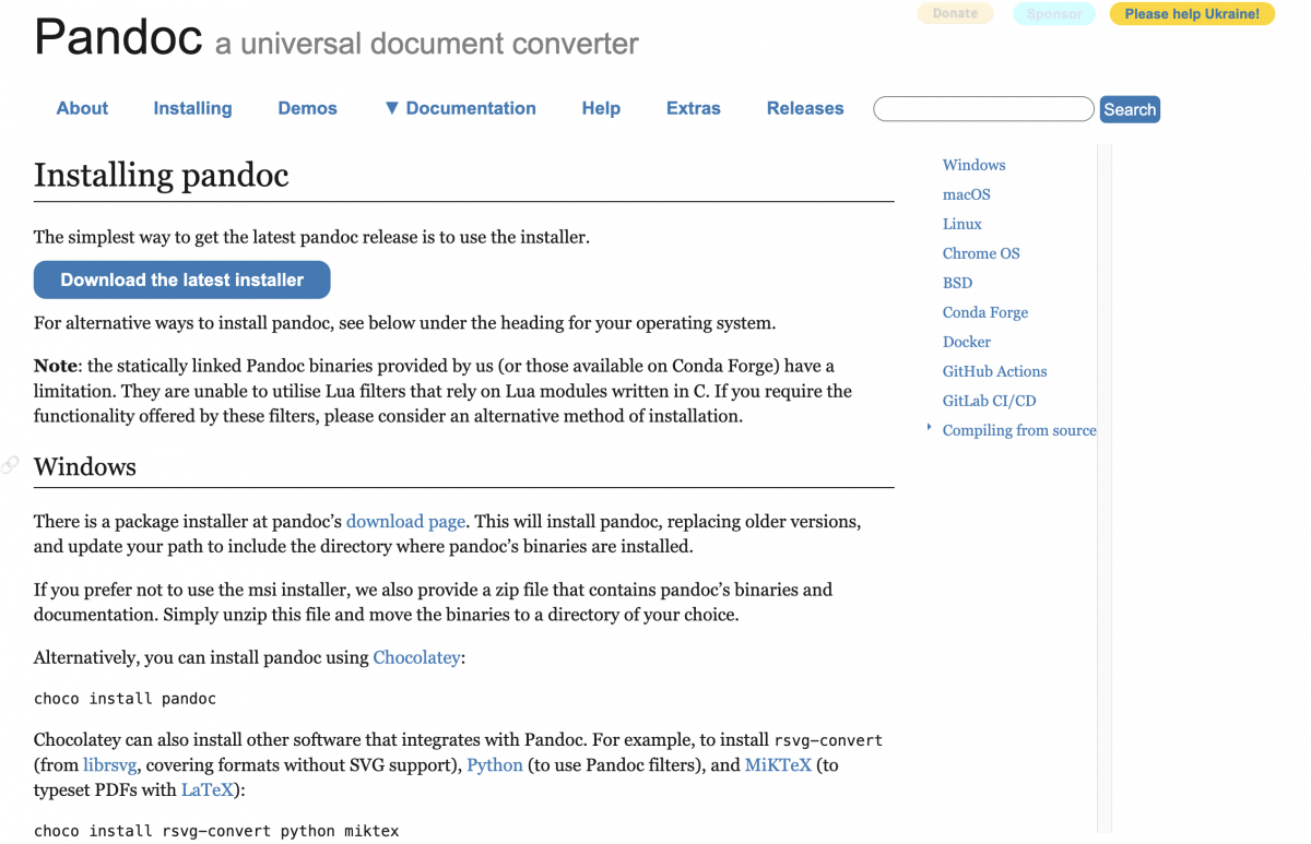
1. Installing Pandoc on Windows
- Start on pandoc.org, not an unofficial download site. Then navigate to “Installing” in the topnav.
- For Windows beginners, choose the .msi installer because it handles setup automatically.
- Avoid the .zip option for beginner instructions unless a manual install is required.
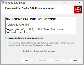
2. Run the Windows Installer
- Accept the license agreement, then click Install.
- The default per-user install is usually enough and does not require administrator privileges.
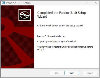
- After the installer finishes, close and reopen Command Prompt before testing Pandoc.
Accept license
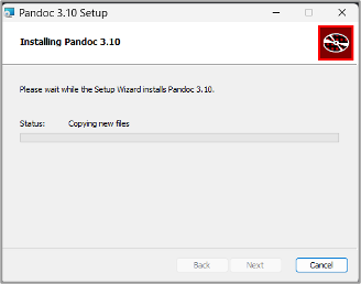
Install progress
Finish setup
3. Verify the installation
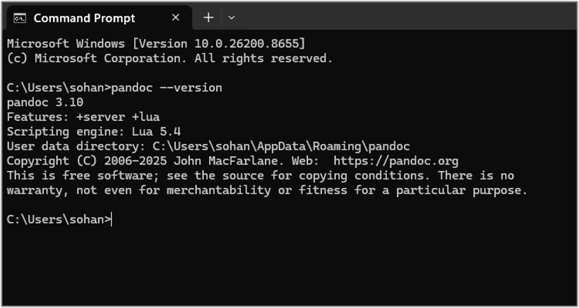
Before proceeding with any LaTeX conversion, confirm that the system recognizes the Pandoc command
- Open a new Command Prompt window after installation.
- Run:
pandoc --version - A version number confirms Pandoc is installed and available on the system path.
- If the command is not found, reopen Command Prompt or restart the computer.
Pandoc Local Installation for macOS
1. Installing Pandoc on macOS
Installing Pandoc using the official download page
Visit Pandoc’s download page for macOS and follow the steps to use the latest package installer on Pandoc’s download page.
Installing Pandoc using Homebrew
Homebrew is a package manager for macOS that can help you easily and quickly download software and packages for your Mac. Read more about Homebrew and how to install it.
Once Homebrew is installed, to install Pandoc using Homebrew, simply open up a new terminal instance and run the following command:
brew install pandoc
2. Verifying the Installation
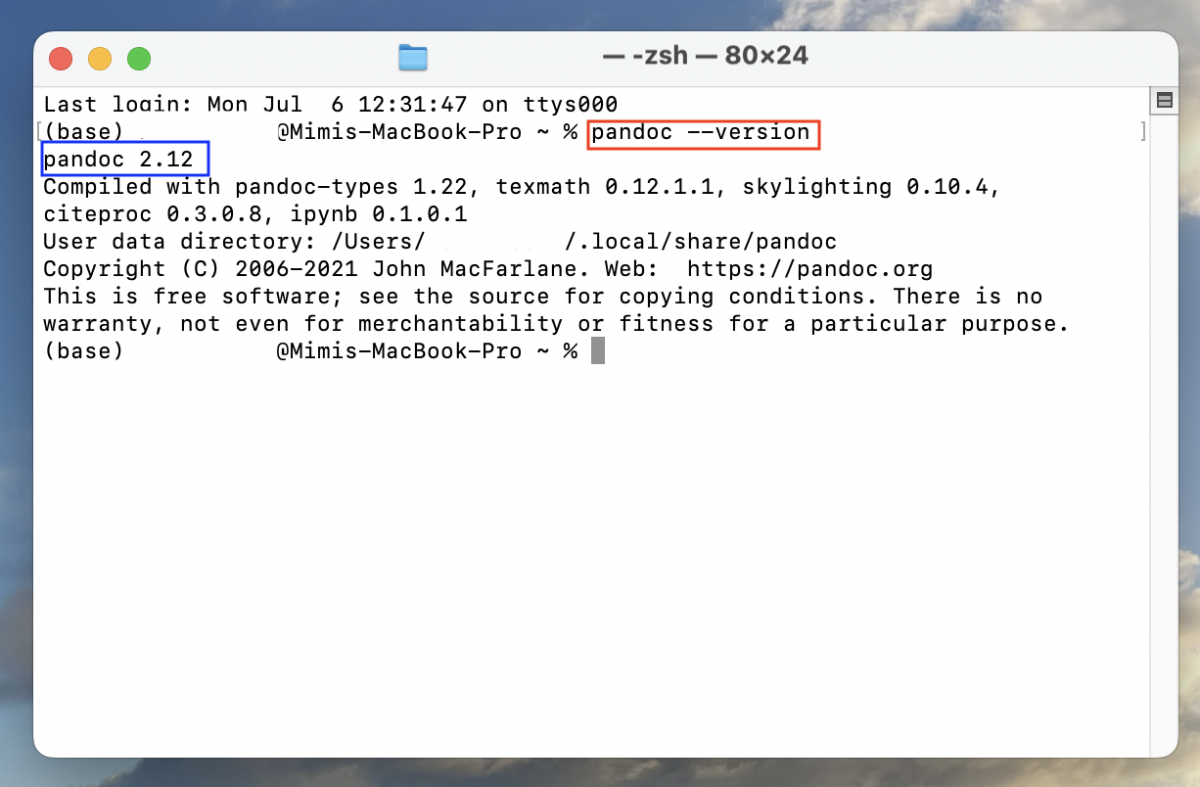
Before proceeding with any LaTeX conversion, confirm that the system recognizes the Pandoc command
- Open a new Terminal window after installation.
- Run:
pandoc --version - A version number confirms Pandoc is installed and available on the system path.
- If the command is not found, reopen Terminal or restart the computer.
Prepare the Project Folder
The Pandoc converter needs the .tex file and every resource referenced by the LaTeX source. The following section applies to LaTeX project folders in both Windows and macOS.
- Keep the .tex file and the figures folder together in one project folder.
- Use relative image paths in LaTeX, such as figures/stability_plot.png.
- Do not rename image files after writing the LaTeX source.
- For Windows: make sure to turn on File name extensions in order to confirm that the file is a .tex
Note that if the path in LaTeX does not match the folder, the image will not appear in the converted HTML.
Example:

The LaTeX command \includegraphics{figures/stability_plot.png} requires a real figures folder with that exact file name, as seen on the left.
Convert LaTeX to HTML5 With MathML
Once the project structure is prepared per the above, you can start using Pandoc locally to convert your LaTeX resources into accessible HTML5 for use with NVDA.
Note: before running any commands, ensure that you cd into the correct directory via Command Prompt on Terminal where your .tex LaTeX source files and supplemental resources in the project folder are located. (Example: cd /Users/Myriam/Library/CloudStorage/OneDrive-UniversityofConnecticut/Documents/latex/)
If you are cd’ing into UConn OneDrive, note that the folder paths often contain spaces. The following is an example cd command into onedrive: cd "C:\Users\sohan\My Drive\UCONN\ITS STEM LATEX\Documents to be shared\accessible_latex_nvda_demo_standalone\accessible_latex_nvda_demo"
LaTeX to HTML5 using Pandoc on Windows
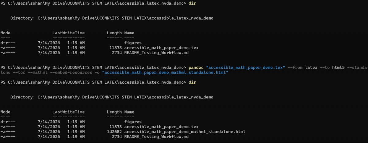
Use the following local conversion command in Command Prompt, replacing accessible_math_paper_demo.tex with your .tex original LaTeX source document, and accessible_math_paper_demo_mathml_standalone.html with the desired name for your new output HTML5 file:
pandoc "accessible_math_paper_demo.tex" ^
  --from latex --to html5 --standalone --toc --mathml --embed-resources ^
-o "accessible_math_paper_demo_mathml_standalone.html" -screates a full standalone HTML document.--toccreates a linked document index/table of contents.--mathmlconverts LaTeX equations into MathML.--embed-resourcesembeds images into the HTML file.-onames the output file.
LaTeX to HTML5 using Pandoc on macOS
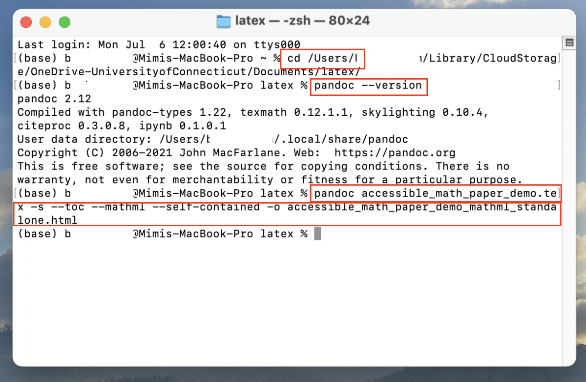
In Terminal, first run pandoc --version to determine which command you will use for the conversion.
If you have Pandoc version 2.19 or newer
Use the following local conversion command in Terminal, replacing accessible_math_paper_demo.tex with your .tex original LaTeX source document, and accessible_math_paper_demo_mathml_standalone.html with the desired name for your new output HTML5 file:
pandoc accessible_math_paper_demo.tex -s --toc --mathml --embed-resources -o accessible_math_paper_demo_mathml_standalone.html
If you have a Pandoc version older than 2.19
Use the following local conversion command in Terminal, replacing accessible_math_paper_demo.tex with your .tex original LaTeX source document, and accessible_math_paper_demo_mathml_standalone.html with the desired name for your new output HTML5 file:
pandoc accessible_math_paper_demo.tex -s --toc --mathml --self-contained -o accessible_math_paper_demo_mathml_standalone.html
-screates a full standalone HTML document.--toccreates a linked document index/table of contents.--mathmlconverts LaTeX equations into MathML.--embed-resourcesembeds images into the HTML file for Pandoc versions 2.19+.--self-containedembeds images into the HTML file for Pandoc versions older than 2.19.-onames the output file.
LaTeX to HTML5 using Pandoc on the Web (not recommended)
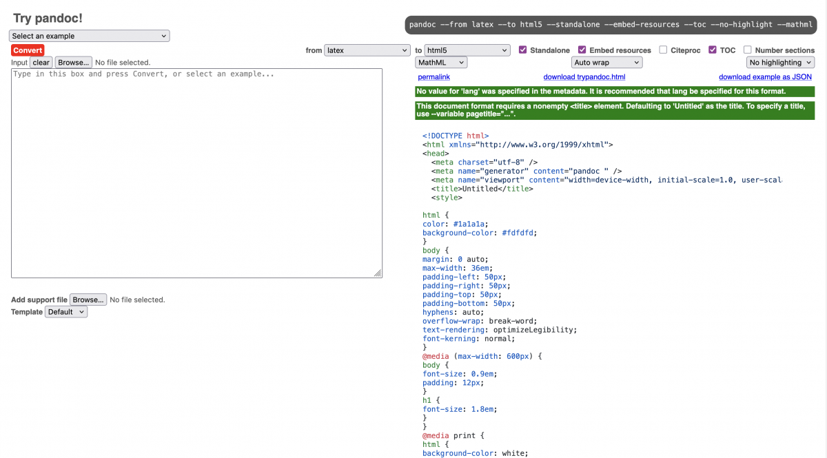
You can also use Pandoc on the web to convert, although it is not recommended because it is not able to integrate images or figures. Additionally, online tools should not be used for confidential/unpublished research without approval. For privacy purposes it is better to use the local versions mentioned above (for Windows and macOS). However, Pandoc online can be useful for simple, math-only examples.
Use the following link to access Pandoc on the web.
- Select from: LaTeX and to: HTML5.
- Check Standalone and TOC.
- Choose MathML for math output.
- Paste LaTeX or upload a simple .tex file.
- If figures do not load, the uploaded file names and image paths likely do not match.
Note on MathML vs. MathJax for the output:
MathML HTML (Recommended)
- Recommended first output for NVDA testing.
- Math is embedded semantically in the HTML.
- Works well with NVDA 2026.1.1 in our test.
- Use –mathml in Pandoc.
- Select MathML for math output on Pandoc on the web
MathJax HTML
- Useful comparison output for visual rendering.
- Often depends on JavaScript and internet access unless configured locally.
- Screen reader behavior can vary by browser and settings.
- Use –mathjax in Pandoc.
- Select MathJax for math output on Pandoc on the web
Setting up NVDA
Once the LaTeX has been converted to HTML5, the NVDA screenreader can be used for testing its accessibility.
Note: NVDA is only available on Windows and incompatible with macOS at this time. For more information on testing NVDA on a Mac and possible workarounds, see here.
NVDA Setup for Testing
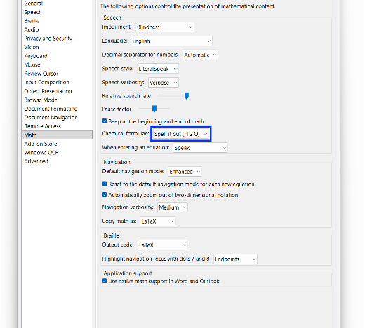
Once installed, note the following settings and instructions for NVDA:
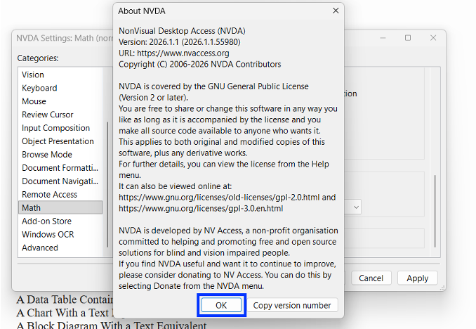
- Use NVDA 2026.1.1 or later.
- Math speech style: ClearSpeak.
- Speech verbosity: Medium.
- Use Firefox first, then Chrome if needed.
- Keep Browse Mode active on the HTML page.
NVDA Testing Shortcuts
Document structure
- NVDA + Down Arrow: continuous reading
- H / Shift + H: next or previous heading
- Tab / Shift + Tab: index links
- NVDA + F7: list headings and links
- G: graphics/images
Math and tables
- T / Shift + T: next or previous table
- Ctrl + Alt + Arrow keys: table cells
- NVDA + Alt + M: math navigation
- Arrow keys: move inside math
- Escape: leave math navigation
NVDA Testing Checklist
- Document Index links jump to the correct sections.
- Heading navigation follows the intended structure.
- Continuous reading moves from text into math and back to text.
- Inline and display equations are read meaningfully.
- Matrices, cases, Greek symbols, and inequalities are understandable.
- Tables can be navigated by rows and columns.
- Images, captions, and long descriptions are read in order.
- The output works in Firefox and is checked in Chrome if possible.
Converting HTML5 to PDF
Once your LaTeX has been converted to HTML5 and successfully tested with NVDA, you can then convert the HTML5 files to PDF for distribution. The following instructions can be used for Windows and macOS:
HTML5 to PDF – Windows
- Open the generated HTML5 file in Chrome, Edge, or Firefox.
- Press Ctrl + P in Windows
- Choose Save as PDF (or Microsoft Print to PDF).
- Keep the page settings as needed, then click Save.
- Open the saved PDF and confirm it looks correct visually.
HTML5 to PDF – macOS
- Open the generated HTML5 file in Chrome, Edge, or Firefox.
- Press Command + P on Mac
- Choose Save as PDF (or Microsoft Print to PDF).
- Keep the page settings as needed, then click Save.
- Open the saved PDF and confirm it looks correct visually.
Troubleshooting the LaTeX Accessibility Workflow
If images do not show
- Confirm the file path matches
/includegraphics. - Run the command from the project folder.
- Use
--embed-resourcesfor a single-file HTML output. - For online conversion, use a ZIP workflow like LaTeXML.
If math does not read correctly
- Confirm the HTML output uses MathML.
- Use NVDA 2026.1.1 or later.
- Use Firefox first.
- Check Math settings: ClearSpeak, Medium verbosity.
- Avoid equation screenshots or unsupported custom macros.
Examples by Discipline
This section will consist of specific accessible LaTeX examples organized by academic discipline. The contents below list the various accessibility examples within the documentation. A PDF version with the list of examples is available, along with the corresponding .tex code for the examples.
Accessibility Examples – Contents
Common LaTeX Elements
- Inline and Display Mathematics
- Fractions, Roots, Exponents, and Subscripts
- Calculus
- Aligned Equations and Multi-Step Derivations
- Vectors and Matrices
- Piecewise Functions and Cases
- Greek Symbols and Control Notation
- Math Inside Lists
- Mathematics in a Data Table
- Chart with a Text Equivalent
- Block Diagram with a Text Equivalent
- Algorithm as Structured Text
Mathematics and Statistics
- Linear Equation With Explicit Steps
- Quadratic Equation by Completing the Square
- Derivative With Separate Left and Right Sides
- Matrix Multiplication
- Proof by Mathematical Induction
- Separate LHS and RHS Trigonometric Derivations
- LHS Derived to a Constant RHS
Computer Science
- Cross-Language Number-Analysis Program
- Python Example
- R Example
- MATLAB Example
- C++ Example
Physics and Astronomy
Physics Examples
- Measurements, Units, and Uncertainty
- Motion with Units and Vector Notation
- Electromagnetic Field Equations
- Quantum-Mechanical Notation
- Tensor and General-Relativity Notation
- Experimental Measurements and Fitted Model
- Experimental-Apparatus Diagram
Astronomy Examples
- Orbital Period and Received Flux
- Distance Modulus and Redshift
- Celestial Coordinates
- Multi-Panel Astronomical Image
- Astronomical Light Curve
- Stellar Spectrum
- Hertzsprung–Russell Diagram
- Astronomical Source Catalog
Engineering
- Electrical Circuit and Kirchhoff’s Current Law
- State-Space and Feedback-Control Models
- Bode Magnitude and Phase Response
- Beam Loading and Free-Body Diagram
- CAD Drawing, Dimensions, and Tolerances
- Material Stress–Strain Response
- Chemical-Process Flow and Recycle Loop
- Robotic Coordinate Frames and Transformations
- Finite-Element Simulation Result
Economics and FInance
- Market Equilibrium and a Per-Unit Tax
- Consumer Choice and Constrained Optimization
- Macroeconomic Identities, Indexes, and Growth Rates
- Econometric Model and Regression Results
- Compound Interest and Project Valuation
- Bond Pricing, Yield, and Duration
- Returns, Portfolio Risk, and the Efficient Frontier
- Option Payoffs and Tail-Risk Measures
- Financial Statements and Ratio Analysis
Linguistics
- International Phonetic Alphabet and Transcription
- Acoustic Phonetics and Vowel-Space Data
- Phonological Rules, Syllables, and an Optimality Tableau
- Morphology and Interlinear Glossed Text
- Judgment Marks, Phrase Structure, and Constituency
- Dependency Syntax and Corpus Annotation
- Formal Semantics, Quantifiers, and Scope
- Pragmatics, Coreference, and Spoken-Language Transcripts
- Signed-Language and Multimodal Annotation
- Historical Linguistics and Language Family Relationships
- Geographic Variation and a Schematic Dialect Map
- Corpus Frequencies and Sociolinguistic Models
Philosophy and Logic
- Logical Symbols, Scope, and Use–Mention Distinctions
- Propositional Logic and Complete Truth Tables
- Natural Deduction and the Scope of a Subproof
- Predicate Logic, Quantifier Order, and Identity
- Categorical Logic and an Euler Diagram
- Sets, Relations, Functions, and a Relation Matrix
- Formal Semantics, Models, and Metalogical Consequence
- Sequents, Proof Trees, and a Semantic Tableau
- Modal Logic and a Possible-World Model
- Modalities Used in Philosophical Logic
- Many-Valued, Fuzzy, and Paraconsistent Logic
- Bayesian Epistemology and Rational Choice
- Argument Maps, Objections, and Replies
- Self-Reference, Quotation, and Defined Predicates
Additional Resources
- Pandoc – Installing Pandoc
- Windows, macOS, Linux, Homebrew, winget, and installer options.
- Pandoc – Getting Started
- Command-line use and terminal instructions for beginners.
- Pandoc Manual
--standalone,--toc,--mathml, and--embed-resourcesoptions.
- LaTeXML Upload Interface
- Converts TeX/LaTeX to HTML5 and accepts a self-sufficient ZIP archive up to 40 MB.
- NV Access documentation
- NVDA math support and MathCAT behavior.
- Accessible LaTeX Examples – PDF
- PDF with accessible LaTeX examples – a list of both common examples and examples by academic discipline.
- Accessible LaTeX Examples – .tex file
- LaTeX source file (.tex) with accessible LaTeX examples – a list of both common examples and examples by academic discipline.